If deaths in each country follows a binomial distribution, how do we rank them by the probability parameter?
Author
Kenneth Hung
Published
February 15, 2020
Introduction
With the coronavirus spreading to many countries, Rebecca asked me a curious question: how does the US perform during SARS compared to other regions in terms of survival rate? While we can compute the survival rate of all infected regions and rank them accordingly, we are ignoring the sampling variability. For example, South Africa that has one case but also one death, does not necessarily perform worse than Indonesia where there were two cases but both patients survived.
Setup
Of course there are many other factors, but we can consider an idealized model where the number of patients, \(n_i\) in each country is predetermined, but the number of deaths, \(X_i\) is random and comes from a binomial draw: \[X_i \sim \text{Binomial}(n_i, p_i),\] where \(p_i\) represent the chance of a patient dying in region \(i\). We would then want to provide simultaneous confidence intervals for the rank of region \(i\), \(r_i\), as defined in Al Mohamad et al. (2022): \[r_i = 1 + \#\{j \ne i: p_j < p_i\}\] There is an obvious Bayesian way to achieve this. By setting up a reasonable prior, we can perform posterior draws of \(p_i\) and search for confidence intervals of ranks that covers \((1 - \alpha)\) of the posterior draws. Naturally this can be extended to an empirical Bayes way as well, as suggested in one of the comments in this Cross Validated thread. We want to focus on strict frequentist methods here.
Data
I have never done data scraping, so I am glad that this led me to learn rvest. We read in the table from the SARS page on Wikipedia. It looks like this:
One way is to construct simultaneous confidence intervals for each of the region, and “project” to figure out the ranks. We implement those here:
Show the code
umpu.expfam.test <-function(x, prob, u =runif(1)) { x <- x -min(which(prob !=0)) +1 prob <- prob[min(which(prob !=0)):max(which(prob !=0))] n <-length(prob)if (x > n | x <=0) {return(0) } mean.x <-sum(prob *1:n)# observation is meanif (abs(x - mean.x) < .Machine$double.eps^0.5) {return(1- u * prob[x]) }# observation is on lower tailif (x < mean.x) { x <- n +1- x mean.x <- n +1- mean.x prob <-rev(prob) }# dot product with this vector gives the covariance with x cov.vec <- prob * (1:n - mean.x) prob.hi <-sum(prob[-(1:x)]) + prob[x] * u cov.tail <-sum(cov.vec[-(1:x)]) + cov.vec[x] * u cov.cumsum <-cumsum(cov.vec) + cov.tail lo <-min(which(cov.cumsum <0)) prob.lo <-sum(prob[1:lo]) - cov.cumsum[lo] / cov.vec[lo] * prob[lo] prob.lo + prob.hi}umpu.binom.test <-function(x, n, p, u =runif(1)) {umpu.expfam.test(x +1, dbinom(0:n, n, p), u)}umau.binom.ci <-function(x, n, alpha, u =runif(1)) { f <-function(p) {umpu.binom.test(x, n, p, u) - alpha } tol <- .Machine$double.eps^0.5if (x ==0) { ci.lo <-0 } else { ci.lo <-uniroot(f, c(0, x / n), tol = tol)$root }if (x == n) { ci.hi <-1 } else { ci.hi <-uniroot(f, c(x / n, 1), tol = tol)$root }c(ci.lo, ci.hi)}# delta is the difference in log-oddsumpu.binom.contrast.test <-function(x1, n1, x2, n2, delta =0, u =runif(1)) { log.prob <-dbinom(0:(x1 + x2), n1, 0.5, log =TRUE) +dbinom((x1 + x2):0, n2, 0.5, log =TRUE) +0:(x1 + x2) * delta log.prob <- log.prob -max(log.prob) prob <-exp(log.prob) prob <- prob /sum(prob)umpu.expfam.test(x1 +1, prob, u)}
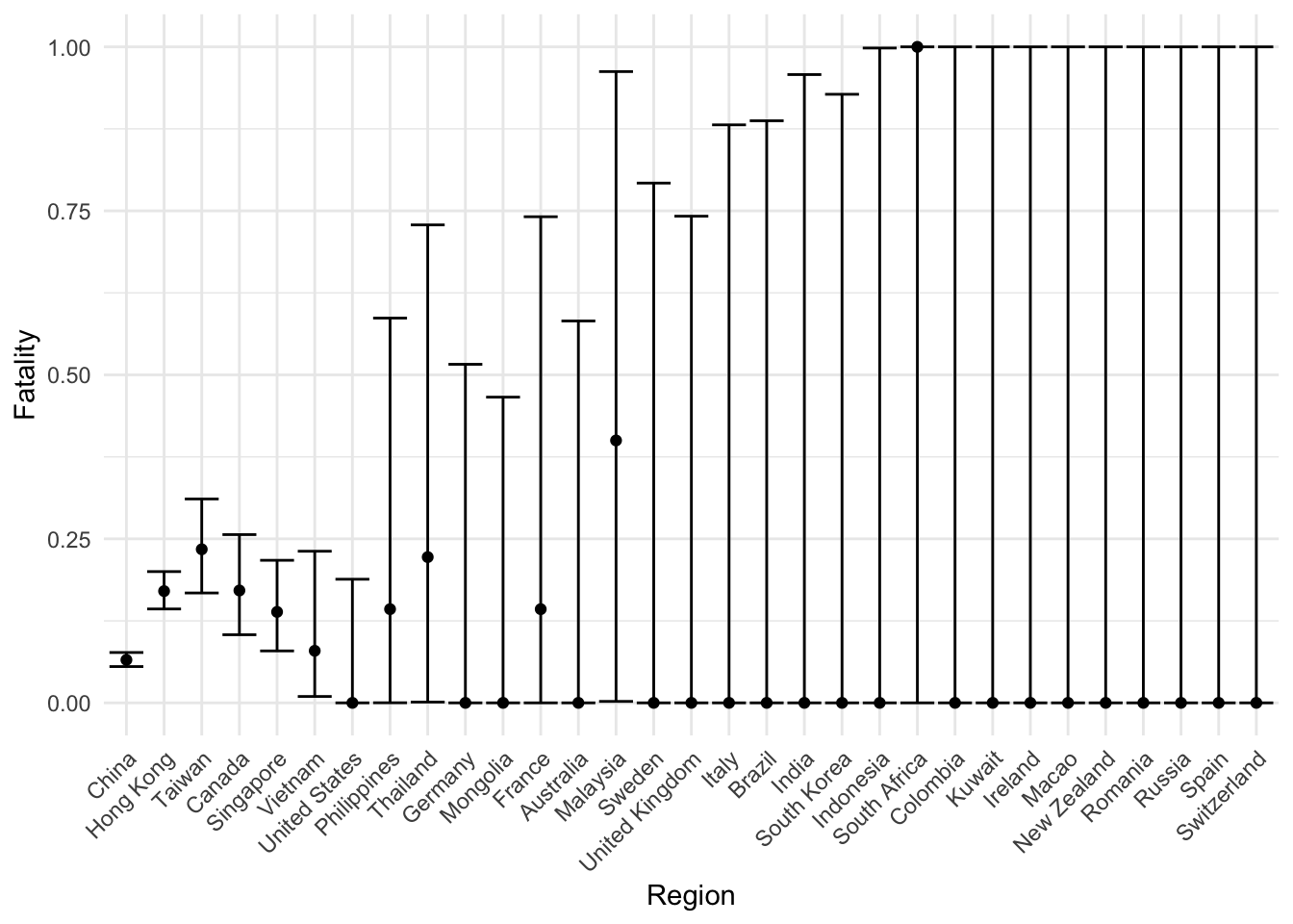
We construct UMAU simultaneous confidence intervals:
set.seed(20200215)data.ci <-mapply( umau.binom.ci, data$deaths, data$cases,MoreArgs =list(alpha =0.05/nrow(data))) %>% t %>% data.frame %>%setNames(c('ci.lo', 'ci.hi'))data <- data %>%cbind(data.ci)ggplot( data,aes(x =factor(region, region), y = fatality, ymin = ci.lo, ymax = ci.hi)) +geom_point() +geom_errorbar() +theme_minimal() +theme(axis.text.x =element_text(angle =45, hjust =1)) +labs(x ="Region", y ="Fatality")
These UMAU intervals are random by nature. Furthermore, the simultaneous coverage is achieved by Bonferroni correction here. A more fine-tuned analysis can be obtain by strategically distribute the type I error over the 29 regions, especially when some of these intervals are likely uninformative.
We can now compute the ranks for all parameters falling into the simultaneous confidence region
data %>%mutate(rank.lo =1+rowSums(outer(ci.lo, ci.hi, FUN ='-') >=0),rank.hi =rowSums(outer(ci.hi, ci.lo, FUN ='-') >=0) ) %>%kbl(format ="markdown")
region
cases
deaths
fatality
ci.lo
ci.hi
rank.lo
rank.hi
China
5327
349
0.0655153
0.0553309
0.0767850
1
27
Hong Kong
1755
299
0.1703704
0.1431314
0.2001229
2
31
Taiwan
346
81
0.2341040
0.1675014
0.3108369
2
31
Canada
251
43
0.1713147
0.1038446
0.2564828
2
31
Singapore
238
33
0.1386555
0.0791824
0.2173352
2
31
Vietnam
63
5
0.0793651
0.0097358
0.2311465
1
31
United States
27
0
0.0000000
0.0000000
0.1884739
1
31
Philippines
14
2
0.1428571
0.0001477
0.5865567
1
31
Thailand
9
2
0.2222222
0.0012364
0.7285998
1
31
Germany
9
0
0.0000000
0.0000000
0.5160983
1
31
Mongolia
9
0
0.0000000
0.0000000
0.4660410
1
31
France
7
1
0.1428571
0.0000000
0.7410531
1
31
Australia
6
0
0.0000000
0.0000000
0.5821487
1
31
Malaysia
5
2
0.4000000
0.0022369
0.9623212
1
31
Sweden
5
0
0.0000000
0.0000000
0.7923318
1
31
United Kingdom
4
0
0.0000000
0.0000000
0.7418809
1
31
Italy
4
0
0.0000000
0.0000000
0.8810932
1
31
Brazil
3
0
0.0000000
0.0000000
0.8873430
1
31
India
3
0
0.0000000
0.0000000
0.9577680
1
31
South Korea
3
0
0.0000000
0.0000000
0.9277255
1
31
Indonesia
2
0
0.0000000
0.0000000
0.9982266
1
31
South Africa
1
1
1.0000000
0.0000000
1.0000000
1
31
Colombia
1
0
0.0000000
0.0000000
1.0000000
1
31
Kuwait
1
0
0.0000000
0.0000000
1.0000000
1
31
Ireland
1
0
0.0000000
0.0000000
1.0000000
1
31
Macao
1
0
0.0000000
0.0000000
1.0000000
1
31
New Zealand
1
0
0.0000000
0.0000000
1.0000000
1
31
Romania
1
0
0.0000000
0.0000000
1.0000000
1
31
Russia
1
0
0.0000000
0.0000000
1.0000000
1
31
Spain
1
0
0.0000000
0.0000000
1.0000000
1
31
Switzerland
1
0
0.0000000
0.0000000
1.0000000
1
31
Method 2: Simultaneous pairwise tests
Binomial distributions is an exponential family, so contrasts like \(p_i - p_j\) are amenable to UMPU tests. We can perform \(\binom{29}{2}\) pairwise tests, with Bonferroni correction, and draw conclusions about the ranks.
Here we are bounded to correct for all \(\binom{29}{2}\) tests, instead of taking advantage of Tukey’s HSD, which incurs a much smaller penalty for multiple testing. Asymptotically we can always think of the likelihood as if it came from a Gaussian distribution and use Tukey’s HSD, but we most definitely are not in any reasonable asymptotic regime here.
Thoughts
Are there better, strictly frequentist methods for computing these rank confidence intervals? This alone seems hard, but there is a natural, even harder generalization of this problem: suppose we have a joint distribution of exponential families where the base measure does not need to be the same \[p_i(X_i; \theta_i) = h(x_i) \exp(\theta_i x_i - A_i(\theta_i)),\] is there a powerful method for ranking \(\theta_i\)?
References
Al Mohamad, D., Goeman, J. J., and van Zwet, E. W. (2022), “Simultaneous Confidence Intervals for Ranks With Application to Ranking Institutions,”Biometric Methodology, 78, 238–247. https://doi.org/10.1111/biom.13419.